[TIL] 데이터분석 데브코스 48일차 (3) - Kaggle 데이터로 SVM, 의사결정나무 모델 활용 머신러닝 실습

 

🔗 실습 링크 : https://www.kaggle.com/datasets/sjleshrac/airlines-customer-satisfaction

Airlines Customer satisfaction

 

 

 

 

 

 

SVM을 활용한 풀이

1단계. 데이터 로드 및 전처리

import numpy as np
import pandas as pd
from sklearn.model_selection import train_test_split

seed = 1234
np.random.seed(seed)

# 데이터 로드
data_path = '/content/Invistico_Airline.csv'
airplane = pd.read_csv(data_path)

• NA값제거
• 지연시간5시간이상제거
• 범주형 데이터 인코딩
• 상관도를 바탕으로 15개 특성 추출
• 20%기준으로 학습 및 평가데이터 분할

# 데이터 자료형에 따른 column 구분

y_column = ['satisfaction']
numeric_columns = ['Age', 'Flight Distance',
                   'Departure Delay in Minutes', 'Arrival Delay in Minutes']
ordinal_columns = ['Seat comfort', 'Departure/Arrival time convenient',
                   'Food and drink', 'Gate location',
                   'Inflight wifi service', 'Inflight entertainment',
                   'Online support', 'Ease of Online booking',
                   'On-board service', 'Leg room service',
                   'Baggage handling', 'Checkin service',
                   'Cleanliness', 'Online boarding']
category_columns = ['Gender', 'Customer Type',
                    'Type of Travel', 'Class']

# na값 제거
airplane_cleaned = airplane.dropna()

# 지연 시간 5시간 이상은 제거
time_limit = 300
airplane_cleaned = airplane_cleaned[(airplane_cleaned['Arrival Delay in Minutes'] < time_limit) &
                                    (airplane_cleaned['Departure Delay in Minutes'] < time_limit)]

# 카테고리형 변수 인코딩
airplane_cate_encoded = pd.get_dummies(airplane_cleaned[category_columns], drop_first=True)
airplane_target_encoded = pd.get_dummies(airplane_cleaned[y_column], drop_first=True)


airplane_combined = pd.concat([airplane_target_encoded,
                               airplane_cleaned[numeric_columns + ordinal_columns],
                               airplane_cate_encoded],
                              axis=1)

# 상관 관계를 바탕으로 15개의 특징만 추출
# 추출할 특징의 이름 ↓
y_column = ['satisfaction_satisfied']
ext_ordinal_columns = ['Inflight entertainment', 'Ease of Online booking',
                       'Online support', 'On-board service',
                       'Online boarding', 'Leg room service',
                       'Checkin service', 'Baggage handling',
                       'Cleanliness', 'Seat comfort',
                       'Inflight wifi service', 'Food and drink']
ext_category_columns = ['Customer Type_disloyal Customer', 'Class_Eco',
                        'Gender_Male']

# 추출된 특징만을 포함할 데이터
ext_airplane_combined = airplane_combined[y_column + ext_ordinal_columns + ext_category_columns]

# 학습 및 평가 데이터 분리
X = ext_airplane_combined.drop(y_column, axis=1)
y = ext_airplane_combined[y_column]
X_train, X_test, y_train, y_test = train_test_split(X, y,
                                                    test_size=0.2,
                                                    random_state=42)

X_train.info()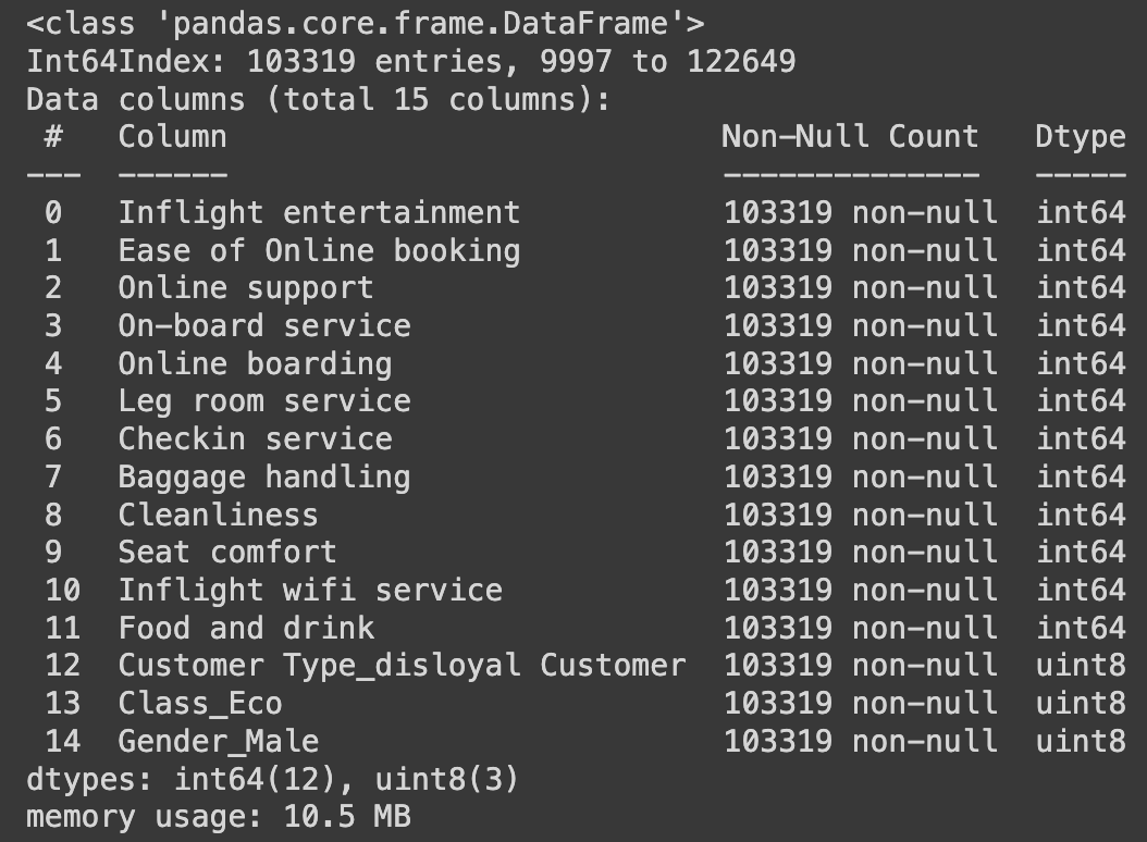

 

 

📌 하나의 셀을 실행시킬 때 얼만큼 시간이 걸렸는지 측정해주는 매직 키워드

%%timeit

 

 

► `854 ms ± 21.5 ms per loop (mean ± std. dev. of 7 runs, 1 loop each)`

• 1개의 루프 안에 7번의 fitting 실행이 있었음
• 약 854 ms 정도의 시간이 걸림

 

 

 

 

2단계. SVM 모델을 활용한 학습

• RBF 커널 사용
• 슬랙 변수 `C = 0.1`로 설정
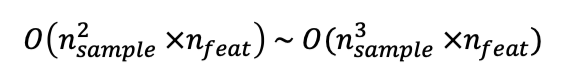
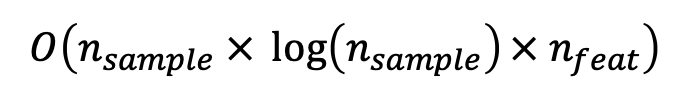
• SVM은 원래 시간이 매우 오래 걸린다. (실습 데이터 기준 약 30분 소요)
• SVM의 시간복잡도 : 

from sklearn.svm import SVC

svm = SVC(kernel='rbf', C=0.1)

%%timeit
svm.fit(X_train, y_train)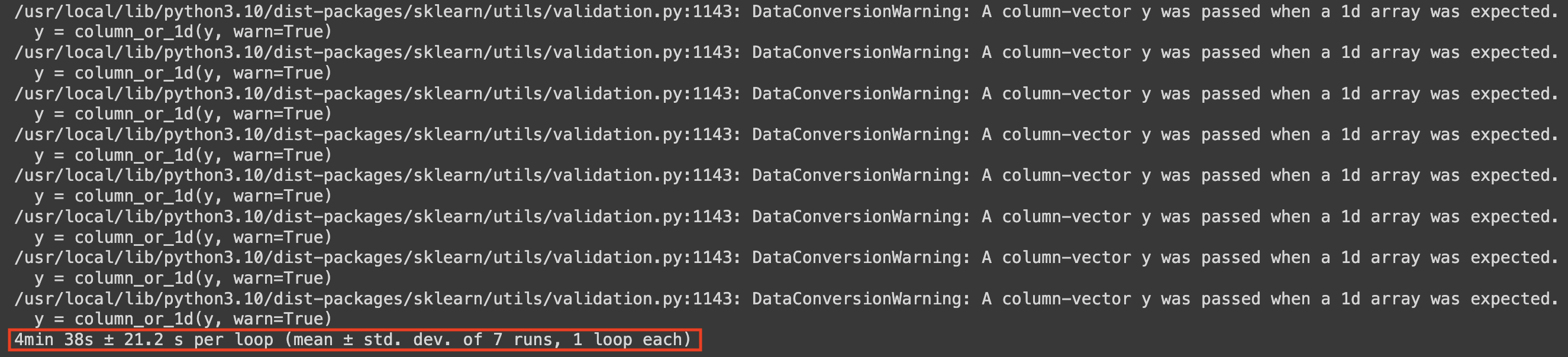

 

 

 

 

 

3단계. 학습 SVM 모델을 활용한 예측 및 평가 진행

# 예측 수행
y_train_pred_svm = svm.predict(X_train)
y_test_pred_svm = svm.predict(X_test)

# 평가 지표 계산: 정확도 (맞은수/전체)
acc_train = accuracy_score(y_train, y_train_pred_svm)
acc_test = accuracy_score(y_test, y_test_pred_svm)

print(f'학습 데이터를 이용한 SVM Acc 값 : {acc_train*100:.1f}%')
print(f'평가 데이터를 이용한 SVM Acc 값 : {acc_test*100:.1f}%')

 

► 로지스틱 회귀 모델을 사용했을 때 평가 데이터를 활용한 정확도가 82.9% 였던것에 비하면 성능이 매우 향상된 것을 알 수 있다.

 

# confusion matrix을 활용한 평가 결과 확인
cm_test_svm = confusion_matrix(y_test, y_test_pred_svm)

plt.imshow(cm_test_svm, interpolation='nearest', cmap='Blues')
plt.title("SVM Confusion Matrix (Test)")
plt.colorbar()
tick_marks = np.arange(len(np.unique(y_test)))
plt.xticks(tick_marks, np.unique(y_test))
plt.yticks(tick_marks, np.unique(y_test))
plt.xlabel("Predicted Label")
plt.ylabel("True Label")

# 각 셀에 숫자 표시
for i in range(cm_test_svm.shape[0]):
    for j in range(cm_test_svm.shape[1]):
        plt.text(j, i, cm_test_svm[i, j], ha="center", va="center", color="black")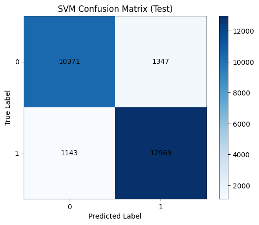

# 정밀도, 재현율, F1 값 비교
from sklearn.metrics import precision_score, recall_score, f1_score

logistic_precision = precision_score(y_test, y_test_pred_logis)
logistic_recall = recall_score(y_test, y_test_pred_logis)
logistic_f1 = f1_score(y_test, y_test_pred_logis)
print(f'Logistic의 P,R,F1 : {logistic_precision:.2f} / {logistic_recall:.2f} / {logistic_f1:.2f}')


svm_precision = precision_score(y_test, y_test_pred_svm)
svm_recall = recall_score(y_test, y_test_pred_svm)
svm_f1 = f1_score(y_test, y_test_pred_svm)
print(f'SVM의 P,R,F1 : {svm_precision:.2f} / {svm_recall:.2f} / {svm_f1:.2f}')

 

► 로지스틱 회귀보다 SVM 모델을 활용한 예측이 훨씬 더 정확하다고  해석할 수 있다.

 

 

 

 

 

 

 

※ 분류 평가 척도 - 정밀도 / 재현율 / F1 점수

1. 정밀도 (Precision)

• 예측한 양성 결과가 실제로 얼마나 진짜 양성인지를 계산
• 모델이 양성 결과를 잘 찾아내야 하는 상황에서 중요

 

2. 재현율 (Recall)

• 실제 양성 중 얼마나 양성을 잘 찾아냈는지를 계산
• 정답을 잘 찾아내는 과정에서 중요

 

※ 정밀도와 재현율은 서로 Trade-off 관계

'(엄청 신중하게)이것은 정답일 수 밖에 없다.' 라고 판단한 것들만 양성이라고 얘기하면 정밀도는 늘어난다.
반면, 재현율은 떨어진다. (∵ 딱 봐도 정답인데 정답이라고 안하고 신중하게 판단 후에 정답이라고 하니까)

 

 

3. F1 Score

• 정밀도와 재현율의 조화 평균
• 조화평균을 사용해 낮음 점수에 대한 패널티를 늘림
• 정밀도와 재현율이 전반적으로 좋아야 좋은 F1값을 갖을 수 있음

 

 

 

 

 

 

 

 

 

 

Decision Tree를 활용한 풀이

• 엔트로피 결정 경계 사용
• 트리의 최대 깊이 `max_depth = 5`로 설정
• SVM에 비해 학습 속도가 빠름 (트리 깊이에 따라 변동성이 크긴함)
• DT의 시간 복잡도 : 

 

 

1단계. Decision Tree 모델을 활용한 학습

from sklearn.tree import DecisionTreeClassifier

dt = DecisionTreeClassifier(criterion='entropy',
                            max_depth=5,
                            min_samples_split=5)
                            
%%timeit
dt.fit(X_train, y_train)

from sklearn.tree import plot_tree

plt.figure(figsize=(100, 20))
plot_tree(dt, filled=True,
          feature_names=ext_ordinal_columns + ext_category_columns,
          class_names=['satisfied', 'unsatisfied'])
plt.title("Plot of Decision Tree")
plt.show()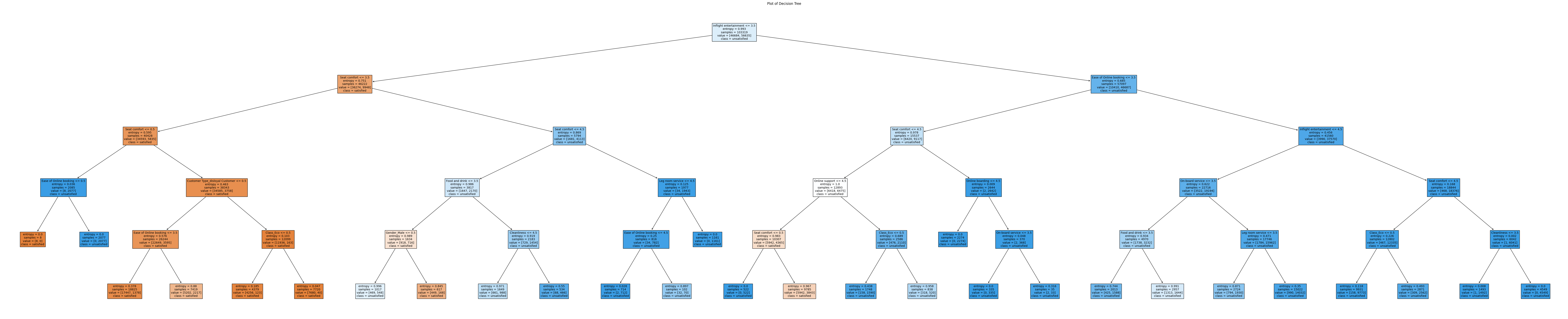

 

 

머신 러닝 모델의 크기가 커지고 복잡도가 증가하면 모델의 성능은 올라간다.

하지만, 과적합이 발생하며 오히려 성능이 하락하기도 한다.

∴ 평가 데이터에 대한 성능이 낮아지기 시작하는 지점의 세팅을 이용해 최적의 모델을 선택하는 것이 바람직하다

 

 

 

 

2단계. max_depth를 조절하면서 최적의 모델 찾기

# max depth에 따른 학습 결과 경향성 파악
max_depths = range(3, 30)

# 훈련 데이터 정확도와 테스트 데이터 정확도를 각각 빈 리스트로 만들고
# for문을 3부터 30까지 돌면서 최고의 모델을 찾는 방식으로 알고리즘 작성
train_accuracies = []
test_accuracies = []

for depth in max_depths:
    model = DecisionTreeClassifier(criterion='entropy',
                                   max_depth=depth,
                                   min_samples_split=5)
    model.fit(X_train, y_train)

    # 학습 데이터에 대한 정확도
    y_train_pred = model.predict(X_train)
    train_acc = accuracy_score(y_train, y_train_pred)
    train_accuracies.append(train_acc)

    # 평가 데이터에 대한 정확도
    y_test_pred = model.predict(X_test)
    test_acc = accuracy_score(y_test, y_test_pred)
    test_accuracies.append(test_acc)

# 결과 시각화
plt.figure(figsize=(10, 6))
plt.plot(max_depths, train_accuracies, label='Training Accuracy')
plt.plot(max_depths, test_accuracies, label='Test Accuracy')
plt.xlabel('Max Depth')
plt.ylabel('Accuracy')
plt.title('Decision Tree Accuracy vs Max Depth')
plt.legend()
plt.show()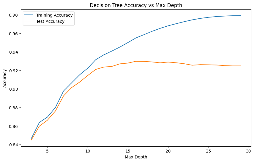

# 최대 정확도를 달성하는 max_depth를 찾고 해당 depth로 최적 모델 학습
max_acc = max(test_accuracies)
best_depth = max_depths[test_accuracies.index(max_acc)]
print('최대 정확도의 depth :', best_depth)

dt = DecisionTreeClassifier(criterion='entropy',
                            max_depth=best_depth,
                            min_samples_split=5)

 

# 예측 수행
y_train_pred_dt = dt.predict(X_train)
y_test_pred_dt = dt.predict(X_test)

# 평가 지표 계산: 정확도 (맞은수/전체)
acc_train = accuracy_score(y_train, y_train_pred_dt)
acc_test = accuracy_score(y_test, y_test_pred_dt)

print(f'학습 데이터를 이용한 DT Acc 값 : {acc_train*100:.1f}%')
print(f'평가 데이터를 이용한 DT Acc 값 : {acc_test*100:.1f}%')

 

► 최적의 `max_depth = 16` 인 것을 찾고 이를 모델에 적용 시킨 결과, 정확도가 확연히 높아진 것을 알 수 있다.

 

# confusion matrix을 활용한 평가 결과 확인
cm_test_dt = confusion_matrix(y_test, y_test_pred_dt)

plt.imshow(cm_test_dt, interpolation='nearest', cmap='Blues')
plt.title("Decision Tree Confusion Matrix (Test)")
plt.colorbar()
tick_marks = np.arange(len(np.unique(y_test)))
plt.xticks(tick_marks, np.unique(y_test))
plt.yticks(tick_marks, np.unique(y_test))
plt.xlabel("Predicted Label")
plt.ylabel("True Label")

# 각 셀에 숫자 표시
for i in range(cm_test_dt.shape[0]):
    for j in range(cm_test_dt.shape[1]):
        plt.text(j, i, cm_test_dt[i, j], ha="center", va="center", color="black")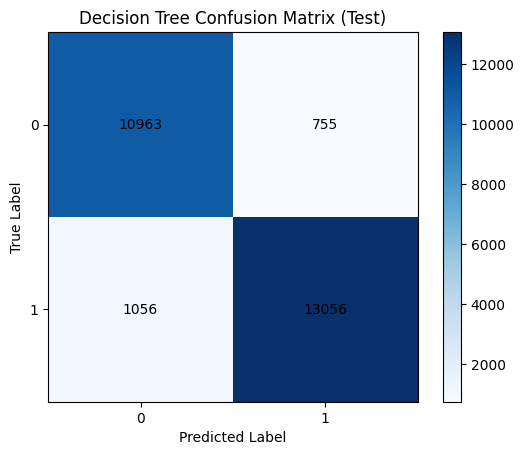

 

 

 

 

 

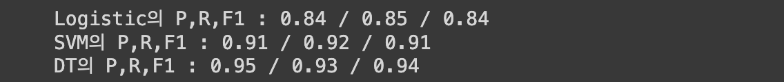
3단계. 각각 로지스틱, SVM, DT를 활용했을 때의 성능 비교해보기

# 정밀도, 재현율, F1 값 비교
from sklearn.metrics import precision_score, recall_score, f1_score

logistic_precision = precision_score(y_test, y_test_pred_logis)
logistic_recall = recall_score(y_test, y_test_pred_logis)
logistic_f1 = f1_score(y_test, y_test_pred_logis)
print(f'Logistic의 P,R,F1 : {logistic_precision:.2f} / {logistic_recall:.2f} / {logistic_f1:.2f}')


svm_precision = precision_score(y_test, y_test_pred_svm)
svm_recall = recall_score(y_test, y_test_pred_svm)
svm_f1 = f1_score(y_test, y_test_pred_svm)
print(f'SVM의 P,R,F1 : {svm_precision:.2f} / {svm_recall:.2f} / {svm_f1:.2f}')


dt_precision = precision_score(y_test, y_test_pred_dt)
dt_recall = recall_score(y_test, y_test_pred_dt)
dt_f1 = f1_score(y_test, y_test_pred_dt)
print(f'DT의 P,R,F1 : {dt_precision:.2f} / {dt_recall:.2f} / {dt_f1:.2f}')